Coupled pressure and saturation prediction for two-phase flow in porous media using physics-informed neural networks (PINNs)
The question
Why can a neural network get the pressure right and still put the water in the wrong place?
When water is pumped into oil-bearing rock, pressure drives the water, and the water changes how easily both fluids move. Pressure varies smoothly, but water saturation, the fraction of pore space filled with water, jumps sharply at the front. Physics-informed neural networks are known to blur such jumps, and earlier studies avoided the coupled problem by predicting the water alone or splitting the work. We trained one network on both equations at once and asked what it needs to get both right.
What we found
Without additional smoothing, the network could approximate pressure well while smearing and misplacing the water front, with saturation error more than ten times the pressure error. Across 658 training runs, increasing network size, adding training points, and reweighting losses did not resolve this difficulty. Introducing a small artificial diffusion term improved the front prediction; combining it with tuned loss weights reduced saturation error by about 31% and pressure error by about 59% compared with diffusion alone.
Schematic overview
Learning pressure and water distribution together
Start with water displacing oil
Water enters a rock filled with oil. The amount of water changes sharply at the advancing front, while pressure changes more smoothly.
Predict the connected quantities together
At each position and time, one network predicts pressure and water saturation. Training checks both outputs against the flow equations that connect them.
Adjust how the model learns
We tested smoothing and the relative importance of the equations, starting conditions, and boundary conditions. We checked the resulting predictions against a numerical solver.
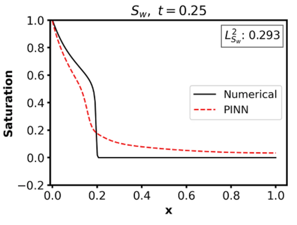
Weighting alone misses the front
Read left to right along the rock. The vertical axis is the water-filled fraction of the pores. The red prediction spreads the water too far ahead of the sharp black reference front.
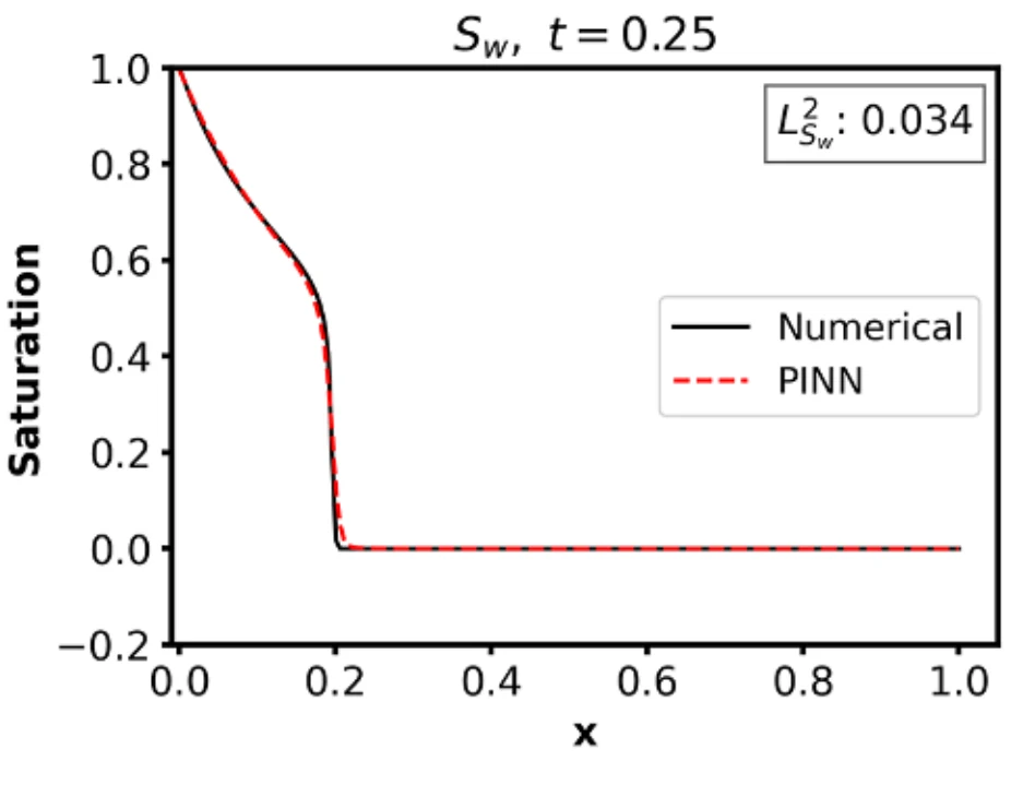
Smoothing and weighting improve the fit
At the same time, the revised model follows the reference front much more closely. Its relative error is 0.034. This is a selected run, not an average over repeated training.
Figure details and test conditions
Both panels use dimensionless position x from 0 to 1 and time t = 0.25. Black is the numerical reference; red dashed is the PINN. Both networks have 10 hidden layers with 50 neurons each and use 450 starting/boundary points plus 10,000 interior points. The left run has no artificial diffusion and weights only the saturation terms (15, 1, 1). The right adds diffusion 0.0035 and weights both fields’ starting, boundary, and equation terms (10, 10, 5). The comparison shows the combined changes, not the effect of either change in isolation.
Learning the pressure and saturation equations together
The pressure equation and the saturation equation behave very differently. Pressure is smooth, and at each moment it depends on where the water is across the whole rock. Water saturation moves with the flow, and in the Buckley–Leverett model its front steepens into a jump. A physics-informed network learns by reducing equation errors at many points, but a jump has no ordinary derivative to check. Networks built from smooth functions also represent jumps poorly. Fuks and Tchelepi found that such networks failed on the saturation equation alone unless a little diffusion was added.
Training on the coupled system also requires a single loss to balance two equations whose errors differ in size and behaviour. A model can therefore fit pressure well while still placing the water front incorrectly. Earlier physics-informed studies of this flow sidestepped the coupling. Most solved the saturation equation with the flow prescribed. Others gave each field its own network, as Hanna et al. did for a simpler sharp-interface model, or added simulated training data, or stepped through time with a numerical scheme. We tested the simplest coupled design: one network with two outputs, trained only on the equations and the starting and boundary conditions.
How training choices affected the water front
Interior training points are locations where we check the equations; they are not measurements from a reservoir. We first tried the usual remedies: larger networks, more training points, and different weights for the equation, starting, and boundary terms. None of them moved the front into place, and in three weighting runs the gradients exploded and training failed.
Adding artificial diffusion improved the predicted front. This numerical smoothing term changes the equation used for training and is separate from the physical properties of the two fluids. As we increased it, the training loss kept falling, reaching its lowest value at the largest setting tested. The saturation error, however, was lowest at a diffusion of 0.0035 (0.041) and reached 0.51 at 0.1. The training loss therefore can’t choose the setting; only comparison with a reference solution can.
Scope of the study
These are one-dimensional tests with uniform rock and no gravity or capillary forces, checked against a numerical reference solution. Settings were selected from single runs, and the three leading configurations were then repeated with three random seeds each. For a forward problem this simple, conventional solvers remain the practical tool. The value of the study is in what it shows about training a coupled network, which later work extends to capillary pressure and to how the smoothing should be handled.
Methods and numbers
The reference uses an implicit-pressure, explicit-saturation numerical scheme, and training combines Adam and L-BFGS. The diffusion-free baseline had mean relative L2 errors of 0.0252 for pressure and 0.308 for saturation. The selected diffusion-and-weighting configuration reached 0.00403 for pressure and 0.0286 for saturation across seven times. These are about 59% and 31% lower than the best diffusion-only configuration. Repeated with three seeds, its mean saturation error was 0.036 ± 0.009. The study comprises 658 training runs, and a global sensitivity analysis found the diffusion coefficient dominant.