A Systematic Analysis of Physics-Informed Neural Networks for Two-Phase Flow with Capillarity: The Muskat–Leverett Problem
The question
What does one network need to learn pressure and water movement once capillary pressure ties them together?
When water pushes oil through rock, or carbon dioxide pushes brine, surface tension creates a pressure difference between the fluids in every pore. This capillary pressure affects how the front spreads and how much fluid is trapped. Many neural-network studies of the flow leave it out, because it couples the pressure and water equations and makes training harder. We kept it, trained one physics-informed network to predict both pressure and water saturation, and mapped which choices decide whether that works.
What we found
Pressure predictions were more accurate than predictions of the moving water front, so choosing a model by pressure error or final training loss would have favoured models with worse fronts. Networks of 10 layers with 50 neurons performed better than deeper ones, and increasing interior equation checks from 5,000 to 50,000 roughly halved the saturation error. These models still required a numerical smoothing term with capillarity included.
Schematic overview
Learning pressure and water movement with capillary pressure included
Include the pressure between fluids
Represent capillary pressure in the coupled flow equations. It arises from the fluid interface, rather than being an extra smoothing term added only to help training.
Learn two connected flow quantities
One network predicts pressure and water saturation together. Pressure drives water movement; the changing fluid distribution affects how easily the fluids flow.
Test training choices against a solver
Vary network size and training-point density, then compare each prediction with a numerical flow solution. Check the moving front, not just the smoother pressure field.
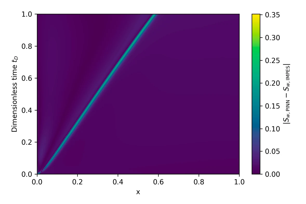
Where the water prediction differs
This is an error map, not an image of rock. Position runs left to right; dimensionless time runs upward. The brighter diagonal follows the moving front, where the network differs most from the numerical reference.
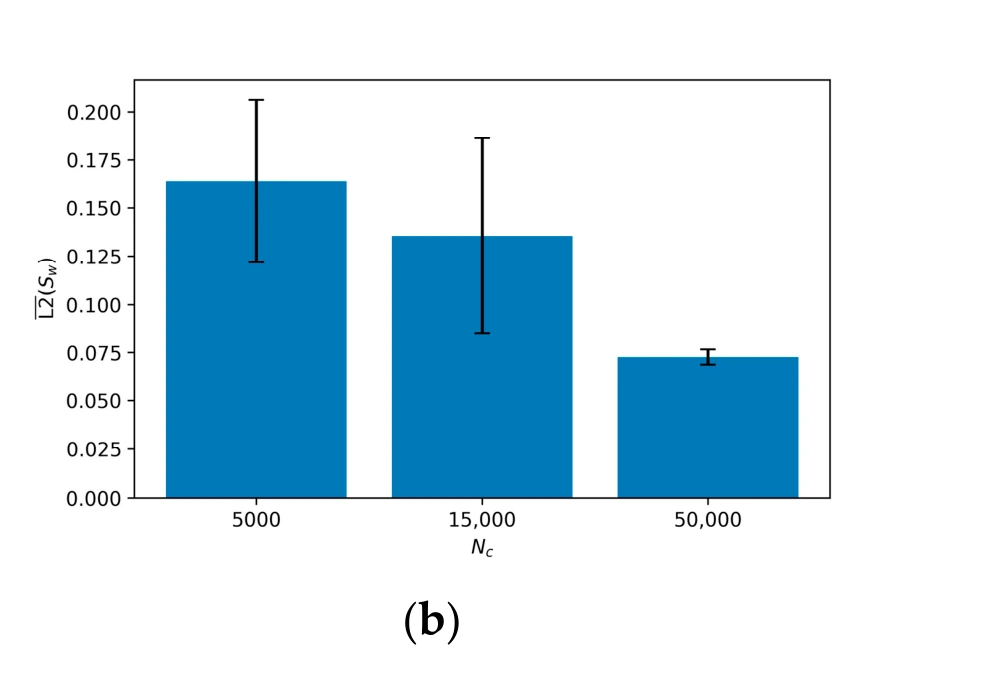
What denser equation checks changed
The horizontal axis counts points where the flow equations are checked during training. The bars show mean relative error in water saturation. The grouped comparison falls as interior points increase from 5,000 to 50,000; lower is better.
Figure details and test conditions
The error map is the baseline case at viscosity ratio M = 3. Its colour measures an absolute difference in saturation, which ranges from zero to one. The bar chart comes from the data-density sweep with 10 layers, 50 neurons per layer, M = 3, and numerical diffusion coefficient 0.0035; it measures relative error instead. All comparisons use simulated flow and the IMPES numerical reference. Physical capillary pressure is included, but the PINN also retains a small artificial diffusion term for training stability.
Figure 3a, PDF page 14; Figure 7b, PDF page 19 from the paper (opens in a new tab)
Why capillarity matters for this flow
When one fluid pushes another through rock, surface tension acts in every pore. The resulting pressure difference between the fluids, capillary pressure, spreads the front in real rock and holds some of the displaced fluid in place. In carbon dioxide storage, this capillary trapping holds at least 10%, and more typically about 30%, of the pore volume as disconnected CO2 (Krevor et al., 2015). In oil recovery, capillary forces drive water into the rock on their own, a process called imbibition.
Most physics-informed studies of two-phase flow instead solve the Buckley–Leverett equation, which drops capillarity and treats the flow velocity as fixed. Keeping capillarity means solving the coupled Muskat–Leverett system. Pressure then depends on saturation through both mobility and a capillary term, and saturation moves with the pressure gradient. The capillary law we used also becomes singular as water saturation approaches zero, which can make training unstable just ahead of the front. Earlier work with capillary pressure studied steady states, or used separate networks for each field to recover flow properties in a fractured rock core. We trained one shared network on the transient coupled system and mapped systematically what it needs.
Physical capillarity and numerical smoothing
We retained the physical capillary term in the pressure equation and added artificial diffusion to the saturation equation to stabilise training. The added diffusion is a numerical smoothing term with a different role from capillary pressure, and it was still needed in these tests even with physical capillarity included. Larger values of that term made the saturation error worse, and the smallest value tested led to severe optimisation failures.
How training choices affected accuracy
The network learned from the governing equations and the starting and boundary conditions, without example solutions as training data. We evaluated its predictions against a reference supplied by the conventional IMPES solver. Networks of 10 layers with 50 neurons each beat deeper ones, and the 30-layer networks became unstable. Increasing the interior equation checks from 5,000 to 50,000 roughly halved the saturation error, while extra boundary data helped much less. For the stiffest cases, a bounded output kept predicted saturation between zero and one.
Across every regime, pressure error stayed about an order of magnitude below saturation error. The model with the lowest final loss and the one with the best pressure were not the ones with the best water front. Accuracy also varied with the physics: saturation error was lowest at a viscosity ratio of 3 and fell steadily as injection pressure increased.
Scope of the study
This is a one-dimensional study with uniform rock and a fixed capillary-pressure curve. Each physical setting needed its own trained network, and we did not compare speed with the conventional solver. Settings were tuned at a viscosity ratio of 3, which is also where accuracy was highest. The network’s front width reflects numerical smoothing as well as capillarity.
Regime results
Mean relative L2 saturation error was 0.162 at viscosity ratio 1, 0.0752 at 3, and 0.246 at 10. Across injection pressures from 0.15 to 1.0, it fell from 0.190 to 0.051. The baseline network has 10 hidden layers with 50 neurons, diffusion 0.0035, 200 boundary points, and 50,000 interior points. Heterogeneous rock, three-dimensional flow, and rate-dependent capillarity remain outside the tested scope.