Separating Artificial-Viscosity Annealing from the L-BFGS Viscosity in Physics-Informed Neural Networks for Two-Phase Flow
The question
When gradually removing smoothing seems to help a flow model, what is actually doing the work?
Neural networks trained on flow equations struggle with the sharp front where injected water displaces oil. A common approach adds artificial viscosity, a mathematical smoothing term distinct from either fluid’s physical viscosity. Several methods gradually reduce this term during training so that the network begins with a smoother problem and works towards the sharp front. In a two-stage pipeline, that schedule also changes the smoothing used in the final stage, so we wanted to distinguish the effects of those two changes.
What we found
Across 15 paired random starts, the final-stage smoothing level had the clearest effect: lowering it increased overall relative error from about 0.22 to 0.26. When that level was held fixed, we detected no benefit from the earlier schedule. The effect also depended on when the flow was evaluated, since stronger smoothing helped while the front remained inside the region but hurt after it left. Easy-to-hard training sequences showed no detected advantage over controls with the same number of stages.
Schematic overview
Separating the training schedule from the final smoothing level
Separate the two training stages
First train with Adam, then refine with L-BFGS. Keep smoothing constant or decrease it during Adam, and choose the L-BFGS setting independently.
Test every schedule and final setting
Run both schedules with both final smoothing levels. Repeat each combination from the same 15 random starting conditions to separate settings from run-to-run variation.
Check before and after front exit
Compare with the flow’s exact solution while the sharp front remains in the region and after it has passed the outlet. Those are different prediction tasks.
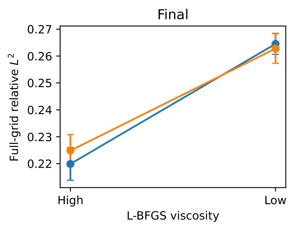
The final setting changes the result
Moving from High to Low final-stage smoothing increases overall prediction error for both earlier schedules. Blue is constant smoothing during Adam; orange is decreasing smoothing. Their small differences at a fixed final setting did not establish a schedule advantage.
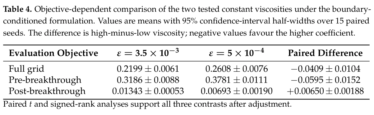
The preferred smoothing depends on when we check
This separate constant-level test compares two smoothing strengths. “Pre-breakthrough” means before the front leaves the region; “post-breakthrough” means after. Lower errors favour stronger smoothing before exit and weaker smoothing afterwards, so an overall score can hide the reversal.
Figure details and test conditions
Both experiments use the one-dimensional Buckley–Leverett model at oil-to-water viscosity ratio 3, with an outlet condition that prevents artificial diffusion through the boundary. Lower relative L2 error means closer agreement with the exact flow. The graph switches from the final Adam state: High = 0.0035 and Low ≈ 0.000167 during L-BFGS. The table is a different constant-level comparison, using 0.0035 and 0.0005 throughout training. Its ± values are 95% confidence-interval half-widths over 15 paired seeds.
Figure 4, first panel (PDF p. 14), and Table 4 (PDF p. 12) from the paper (opens in a new tab)
Understanding the effect of a smoothing schedule
Artificial viscosity makes a sharp water front learnable by smoothing the equation, and several methods reduce it during training. Wassing et al., for example, reduce it to zero during Adam and then continue with L-BFGS at zero. Easy-to-hard training, or curriculum learning, is a standard remedy for hard physics-informed problems more broadly. In an Adam-then-L-BFGS pipeline, though, changing the schedule also changes the smoothing used throughout the second stage. It can also change which saved state is passed between the stages.
If the improvement comes from the final smoothing level, a simpler constant setting may perform equally well. Attributing that improvement to the schedule would make it harder to interpret both the original result and later comparisons that build on it. A review of machine learning for fluid equations found that most studies claiming to beat standard methods compared against weak baselines. This makes the choice of controls important when assessing whether a proposed training method improves on existing approaches.
Designing a controlled comparison
Because variation between random starts can be as large as the effects being measured, a single run provides an unreliable basis for comparison. Changing the smoothing also changes the training equation, so losses at different smoothing levels cannot be used to rank the models directly. The preferred smoothing level can also depend on whether the water front is still inside the region. We crossed each schedule with each final setting, reused the same 15 random starts throughout, and adjusted for multiple comparisons. We also varied the saved state passed between stages and doubled the final training budget. The final-setting effect persisted.
Evaluating the flow before and after front exit
Once the sharp water front passes the outlet, the remaining profile is smooth, and additional smoothing can distort the solution without providing the same training benefit. In our tests, stronger smoothing reduced error before the front left but increased it afterwards. We therefore report errors in both time windows alongside the overall score; evaluating different windows can otherwise lead studies to different conclusions about the preferred setting.
Training on a sequence of increasingly hard flow problems showed no detected accuracy advantage over controls with the same number of stages. Its extra cost came from intermediate stages whose results were discarded.
Scope of the study
These results cover one-dimensional water–oil displacement, one network design, two final smoothing levels, and fixed training budgets. The main experiments add an outlet condition that stops the smoothing term from carrying water out through the boundary. Earlier runs without it showed larger apparent gains, and we report them separately as exploratory. We did not search for an optimal smoothing strength. Conventional finite-volume solvers remain substantially more efficient for this forward problem. Code, configurations, and per-run results are archived on Zenodo.