Performance and stability of physics-informed Kolmogorov-Arnold networks for two-phase transport in porous media: A comparative study with physics-informed neural networks
The question
What does a more compact neural network give up when the flow has a sharp front?
Kolmogorov–Arnold networks, introduced in 2024, learn a small curve on each connection and were promoted for matching larger conventional networks with far fewer parameters. A moving shock is a hard test of that promise: physics-informed networks already struggle where water displacing oil forms a sharp front. We mapped how this design’s settings affect its accuracy and stability on that front, and what its compactness costs.
What we found
Across 2,592 configurations without smoothing, we could not capture the front. Adding artificial smoothing allowed the curve-based network to reach errors of the same order as a conventional network using 1,140 parameters instead of 3,462. This reduction in parameter count required more than twice the smoothing and came with larger early errors near the front and about 50 times longer training, so it did not reduce the computational cost.
Schematic overview
Comparing network size, training time, and the predicted flow
Set up the moving water front
Start with oil in a one-dimensional porous region and inject water at one end. The model must predict how the water fraction changes with position and time.
Change how the network learns
Compare ordinary weighted connections with learnable curves. Both networks are trained to satisfy the flow equation and its initial and inlet conditions.
Check accuracy and computational cost
Tune artificial diffusion, an added smoothing term, to help training. Then check the predicted front, the number of adjustable parameters, and the actual training time separately.
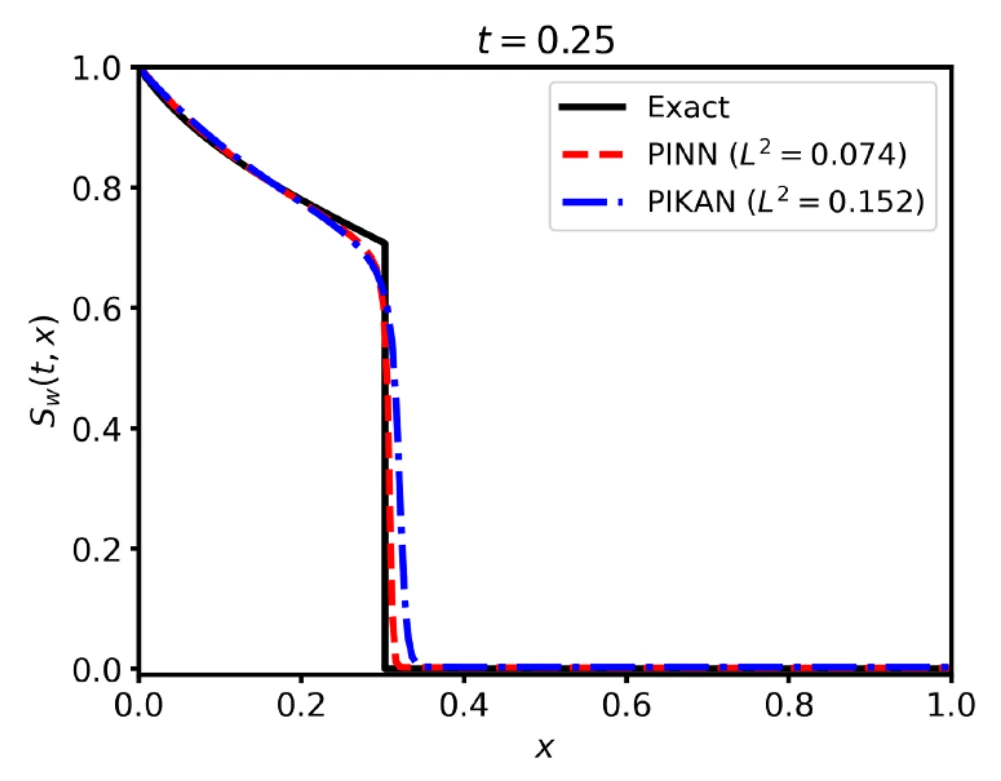
The front at the same moment
Horizontal position runs from inlet to outlet; vertical height is the fraction of pore space filled with water. At time 0.25, the red PINN curve follows the black exact front more closely than the blue PIKAN curve.
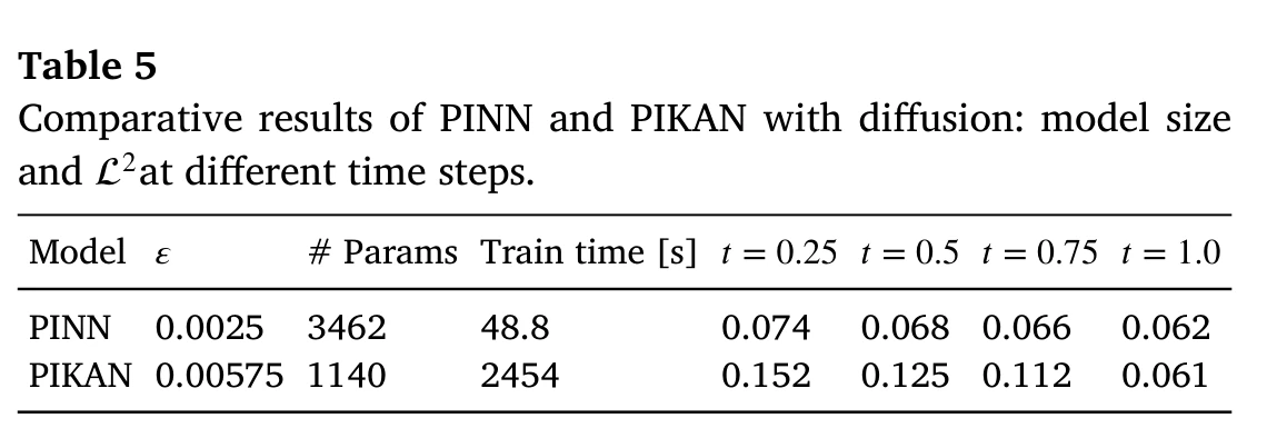
A smaller network took longer to train
Read “# Params” as adjustable values and “Train time [s]” as seconds. PIKAN uses roughly a third as many parameters, yet takes 2,454 seconds versus 48.8. The remaining columns report prediction errors at four times; lower is better.
Figure details and test conditions
These are one-dimensional Buckley–Leverett tests, not field measurements. Black is the exact solution without added diffusion; red is PINN, blue is PIKAN. Each model uses its separately tuned diffusion coefficient: 0.0025 for PINN and 0.00575 for PIKAN. PINN uses 10,000 interior training points and PIKAN uses 50,000, so the timing is specific to these implementations and settings, not an isolated test of architecture alone.
Figure 7, upper-left panel (PDF p. 9), and Table 5 (PDF p. 8) from the paper (opens in a new tab)
Testing a new network on a sharp front
Physics-informed networks blur or misplace the sharp water front in the Buckley–Leverett equation, the classical model of water displacing oil. At the front, water saturation jumps, and the equation has no ordinary derivative to check there. An independent benchmark of remedies found that new network designs left errors close to those of a plain network, while changing the equation or the training reduced them about tenfold. Kolmogorov–Arnold networks were not part of that comparison.
Kolmogorov–Arnold networks, introduced in 2024, learn a small spline curve on each connection instead of using fixed activation functions. They were promoted for reaching similar accuracy with far fewer parameters. Their flexible spline functions were also thought to ease the bias of ordinary networks towards smooth shapes, the bias that makes fronts hard to learn. An earlier application to this equation reported comparable accuracy but much stronger oscillations during training than a conventional network. That left open how the design’s settings affect its stability, and what its compactness costs.
Comparing accuracy, model size, and training time
A smaller model helps when a trained network must be stored or run many times, for example to explore uncertain reservoir properties. It helps less if it needs heavier smoothing or much longer training. We therefore measured adjustable parameters, accuracy against the exact solution, and wall-clock training time separately.
First, we trained 2,592 versions of the physics-informed Kolmogorov–Arnold network (PIKAN) without any smoothing. They varied depth, width, spline order, knot density, and data budgets. None captured the front, so tuning the architecture alone did not solve the problem. The sweep still showed what mattered most: spline order, then knot density and neuron count.
We then added artificial diffusion, a numerical smoothing term, and tuned it separately for each design. We scored the results with four error measures. The best architecture depended on the measure: simple, low-order networks captured the overall solution best, while higher-order networks with dense knots were needed to resolve gradients.
Scope of the study
This is a one-dimensional test with an exact solution for comparison. At the same smoothing level, the conventional network was clearly more accurate.
Errors and settings
With its own tuned diffusion (0.0025 for the PINN, 0.00575 for the PIKAN), relative L2 error at time 0.25 was 0.074 for the PINN and 0.152 for the PIKAN; both reached 0.061 at the final time. At a shared diffusion of 0.0025, average errors were about 0.067 and 0.169. Training took 48.8 seconds for the PINN and 2,454 seconds for the PIKAN. The PINN used 10,000 interior training points and the PIKAN 50,000.