On the Effectiveness of Kolmogorov—Arnold Networks for Enhanced Oil Recovery Prediction in Polymer Flooding
The question
Can a small network with readable parts match a black-box one at predicting oil recovery?
Neural networks can estimate how much oil a polymer flood recovers, but it is hard to see how they reach an answer. Kolmogorov–Arnold networks, or KANs, were proposed as a more transparent alternative: each connection learns a small curve that can be plotted, scored, and pruned. We tested whether a KAN could match our earlier dense network on the same simulated polymer-flooding data, and what its readable structure would reveal.
What we found
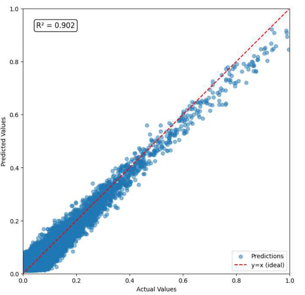
The best KAN reached a test R², a measure of fit, of 0.902 with 1,885 trainable parameters, compared with 0.908 and 43,265 parameters for the dense network. Although its fit was slightly lower, inspecting the KAN’s attribution scores showed that it relied mostly on water saturation, and pruning reduced the calculation to a few dominant pathways.
Schematic overview
Testing predictions and inspecting the fitted model
Learn from simulated reservoir states
The examples include rock properties, pressure, oil and water saturation, oil viscosity, and polymer concentration. The recovery factor is the value to predict.
Fit curves along the connections
A KAN learns a small function on each connection. We varied the network layout, curve resolution, and training method, then checked a held-out 20% of the data.
Inspect which inputs the model uses
Learned curves, attribution scores, and pruned connections expose parts of the fitted calculation, showing which inputs this model relies on.
Prediction compared with the simulation
Each dot compares a predicted recovery factor with its simulated value. The red diagonal marks exact agreement. Points below it are underpredictions; the higher-recovery cases show a visible shortfall.
Water saturation dominates the attribution
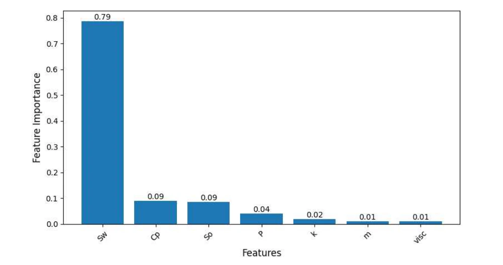
Sw is water saturation: how much of the pore space contains water. It has the largest score in case A1. Cp is polymer concentration; So is oil saturation. The bars show how much the fitted model relies on each input.
Figure details and test conditions
Both figures are from case A1, the best reported KAN, trained with Adam on the synthetic dataset using an 80:20 train/test split. Figure 1 reports test R², a fit statistic rather than a percentage of correct predictions. Figure 4 uses the KAN’s built-in attribution scores. Saturation is an averaged state computed by the simulator, so its importance describes the fitted model rather than the effect of changing a polymer injection.
Figure 1 (PDF p. 4) and Figure 4 (PDF p. 5) from the paper (opens in a new tab)
Inspecting a network’s oil-recovery predictions
Neural networks have been used to predict polymer-flooding and other enhanced-recovery outcomes, often with very high reported fits. For scientific and engineering work, those fits leave a further question: how did the model reach its prediction? Even an accurate network can be difficult to inspect, leaving engineers unable to explain which inputs drove a particular result.
Kolmogorov–Arnold networks, or KANs, were proposed in 2024 as a more transparent alternative. An ordinary network passes signals through fixed activation functions; a KAN learns a small adjustable curve on every connection instead. Those curves can be plotted, scored, and pruned after training. A benchmark on tabular data found KANs accurate, especially on larger datasets, at a higher computational cost. We asked whether that held for predicting oil recovery, and what the readable structure would show.
Training the Kolmogorov–Arnold network
We trained on more than 160,000 simulated samples from our polymer-flooding dataset, using an 80:20 training and test split. Five configurations were trained with Adam for 1,000 steps and five with L-BFGS for 200 steps. They varied the network layout, the resolution of the curves, the spline order, and the learning rate. Adam gave the best fit and the shorter training times. L-BFGS needed fewer steps but took 483 to 2,030 seconds per run, against 124 to 430 seconds with Adam.
Examining the learned connections
The fitted network can be drawn with each connection’s thickness showing its importance. Individual learned curves can be inspected; one first-layer connection, for example, learned a sinusoidal shape. The built-in attribution scores put water saturation far ahead of every other input. Pruning removed the weaker connections and kept the few pathways that carried the prediction.
Scope of the study
The comparison uses the dense network’s score as reported in our earlier study, which used a 70/30 split; that study’s polynomial regression scored slightly higher still (0.909). The inputs include averaged saturations computed by the simulator during the flood, and the dataset study found recovery closely tied to them. Adding physics-based constraints and testing on real-world data are the next steps.
Best configuration
Case A1 has layout [7, 5, 5, 1], spline grid 20, spline order 3, and 1,000 full-batch Adam steps. It reached test mean squared error 0.000597 and test R² 0.902 in 159 seconds of training. The best L-BFGS case reached R² 0.898. Each configuration was a single seeded run.