Identifiability and Conditioning of Flux-Parameter Inversion for the Buckley–Leverett Equation
The question
Which measurements reveal a hidden viscosity ratio, and how much do their errors matter?
Laboratories push water through rock samples and use the measurements to infer how oil and water move. One such property is the viscosity ratio: how much more strongly oil resists flow than water. It sets when water breaks through, so a wrong estimate gives a wrong forecast. Physics-informed networks can estimate such a parameter while reconstructing the flow. We asked what the measurements must contain to determine the ratio, how their errors carry into the estimate, and how much error the network adds.
What we found
For every positive viscosity ratio, the flow equation admits an exact solution, so physics alone cannot select the ratio. Measuring the front speed exactly does determine it, although small speed errors are amplified most when the ratio is small. At a ratio of 3, adding 25 noisy measurements reduced the network’s median error from 514% without observations to about 6%. Further measurements continued to improve the reconstructed water field, without reliably improving the recovered ratio.
Schematic overview
Estimating a viscosity ratio from water movement
Specify the unknown fluid property
Different viscosity ratios produce different water fronts. Each can obey the same flow equation and starting conditions, so physics alone does not select the true ratio.
Determine what observations can reveal
An exact front speed uniquely determines the ratio. With imperfect measurements, recovery also depends on how sensitive the observed flow is to that ratio.
Check the model’s two outputs
Fit a network to simulated observations and the flow equation. Then assess the water distribution and viscosity ratio separately, using their known true values.
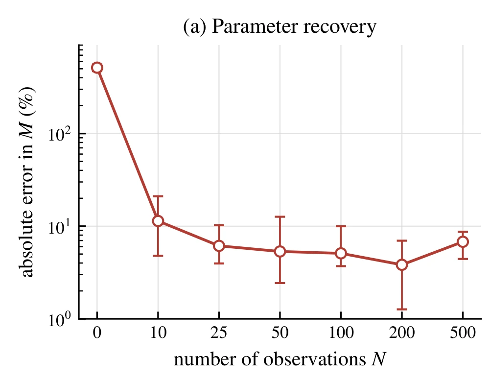
Error in the recovered viscosity ratio
Across the bottom, we add observations. The vertical axis is percentage error in the ratio, on a logarithmic scale. A few observations help greatly; the median does not then fall at every tested count.
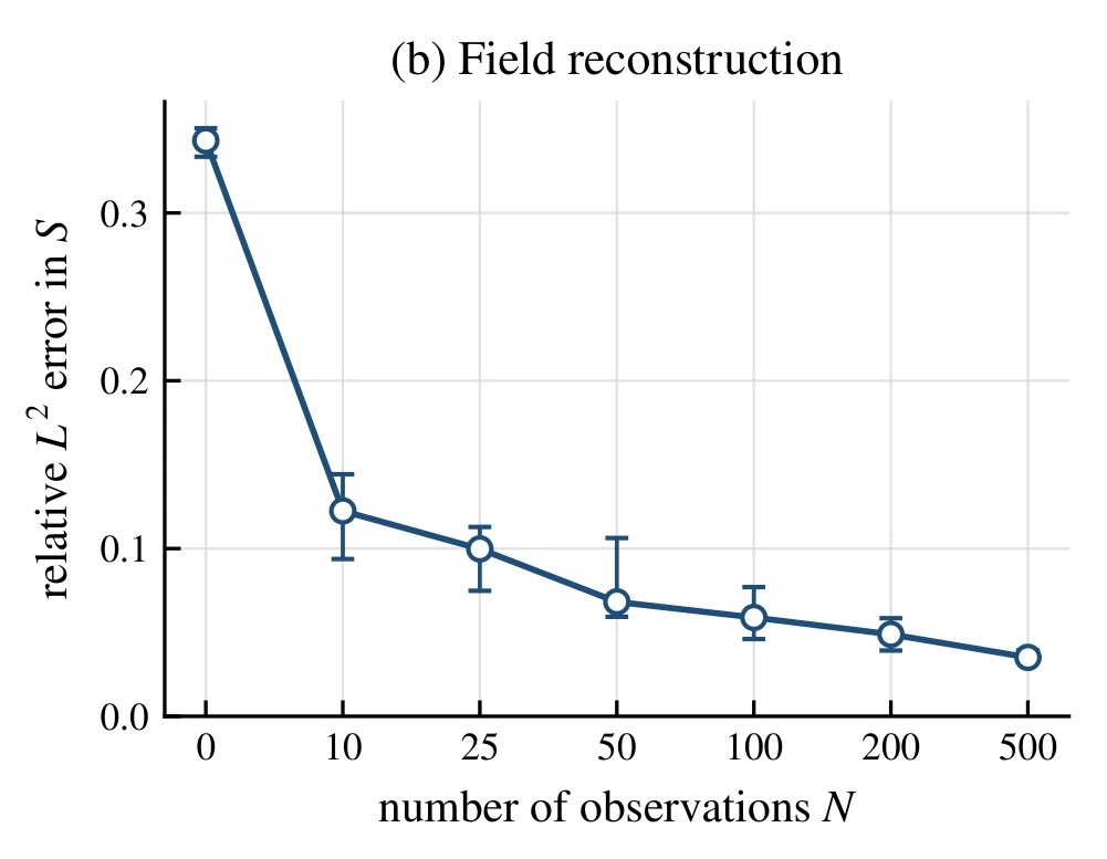
Error in the predicted water distribution
These are the same observation counts and repeated runs. Here the vertical axis measures error across the whole predicted water distribution. Its median falls at every tested count, even where the ratio’s error does not.
Figure details and test conditions
Both panels use a true viscosity ratio of 3, additive Gaussian noise with standard deviation equal to 5% of the saturation range, and the same training budget. Saturation is the fraction of pore space occupied by water. Markers show medians; bars span the middle 50% of 30 paired runs. Lower error is better, but the two vertical axes measure different quantities.
Figure 2a–b, PDF page 13 from the paper (opens in a new tab)
Estimating fluid properties from displacement experiments
Laboratories often read flow properties from displacement experiments. The classic JBN method, for example, does so using the same Buckley–Leverett theory we study (Helset et al., 1998). Those estimates then feed the models used for field forecasts. In our model, raising the viscosity ratio from 3 to 10 brings water breakthrough forward from 0.67 to 0.46 time units. A method that matches measured saturations but returns the wrong ratio would forecast the wrong breakthrough.
To understand why an estimate can be wrong, we need to distinguish what the measurements tell us from the errors introduced when we use them. Identifiability asks whether perfect data would determine a unique answer, while conditioning describes how much that answer changes when the measurements contain a small error. We distinguish both from estimator error: the further error associated with a particular method, such as a neural network. Since these sources of error call for different remedies, separating them is essential to understanding a poor estimate. Mathematical work on recovering the flux in such equations has named the stability of that recovery as an open question (Holden et al., 2014). Earlier neural-network inversions of this equation reported parameter errors without a reference for what accuracy the data could support.
Identifiability and sensitivity to measurement error
With the same starting and boundary conditions, every positive viscosity ratio has an exact solution of the flow equation. A physics-informed network’s physics loss therefore carries no information about the ratio; any preference it shows without data comes from the network and its training. An exact measurement of front speed does fix the ratio, and we derived how strongly speed errors are amplified. A 1% speed error becomes about a 19% ratio error at a ratio of 0.25, but under 3% at a ratio of 10. Measurements scattered through the flow carry different information again, including when the moving front crosses a sensor.
Estimating the ratio with a neural network
We trained a physics-informed neural network to estimate both the water distribution and the ratio from simulated measurements, repeating each main setting 30 times. The first few measurements substantially improved the estimate. As we added more, the reconstructed water field continued to improve, but the recovered ratio did not improve at every step. This is why we assessed both quantities separately: agreement with the observed flow did not, by itself, tell us how accurately the model had recovered the property we wanted to infer. We also compared against a numerical solver without a neural network, to separate smoothing effects from training difficulty.
Scope of the study
The study considers one-dimensional flow with one unknown parameter, using synthetic measurements from the same model family used for the inversion. The network solves a smoothed version of the equation, so it also contends with a mismatch to the sharp front in the data. Its recovery became poorer as that smoothing was reduced, while the solver-based control kept improving.
Numbers and methods
At a true ratio of 3 with 5% Gaussian noise, the median parameter error was 514.25% with no observations, 11.38% with 10, and 6.13% with 25. The front-speed condition number falls from 18.94 at a ratio of 0.25 to 2.86 at 10. Across ratios from 0.25 to 10, median error was largest at the smallest ratio (32.55%). The network uses artificial viscosity to smooth the front, while its measurements come from the exact unsmoothed solution.